Hiding Repeating Values In A Column
When you are working with lists in Excel, you may sometimes find that, after sorting, you have multiple rows with the same values repeating down one or more columns. If you are printing this list as a report, for aesthetic purposes, you may prefer to have only the first instance of each item shown.
One option is to clear the cells for all duplicate items below the first one. The problem with this approach is (a) is can be very time-consuming if you’re working with a long list and (b) once you delete values from the cells, you won’t be able to sort or filter your list.
I sometimes use this Conditional Formatting trick that I need to do only one time. After that, all future duplicate values will be hidden.**(see caveat below)
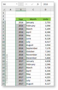
1) Select the range of cells in the column where you want to hide duplicates. In this example we have selected B4:B23. Note that cell B4 is the Active Cell;
2) On the Home tab, click Conditional Formatting in the Styles group and then choose New Rule…;
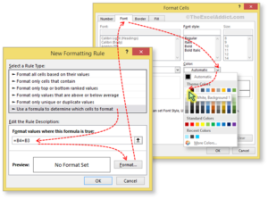
3) Select the Rule Type ‘Use a formula to determine which cells to format‘;
4) With Conditional Formatting, you always base your formula on the Active Cell in the current selection. In this case the Active Cell is B4. So in the formula field type =B4=B3. This formula tells Excel to check if the active cell’s value is equal to cell above. If they are equal, the result of this formula is TRUE, therefore the formatting you specify will be applied to that cell;
5) Click the Format… button, click the Font tab in the Format Cells dialog. Select the Color dropdown, choose white (i.e. the same as the background color of these cells) from the color palette and click OK;
6) Click OK to close the Conditional Formatting dialog.
Since your new Conditional Formatting rule has automatically applied a font color that matches the background color to the duplicate values, those cells will appear blank although the values are still in the cells (just look in the Formula Bar).
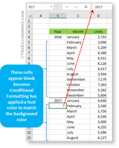
** CAVEAT: Use this trick with caution. Keep in mind that you (or other users of the spreadsheet) may forget that there is data in the ‘seemingly blank’ cells and could cause problems.
Here are a couple of solutions I sometimes use to avoid this:
Solution 1: Make a temporary working copy of the sheet
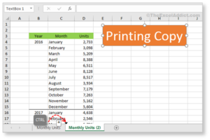
Point to the sheet tab, hold down the CTRL key and drag it to the right. To avoid confusing the two sheets, add a Text box identifying the duplicate sheet. Now your original sheet remains untouched.
Solution 2: Toggle Conditional Formatting On and Off
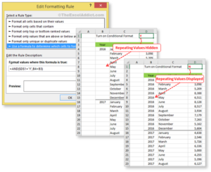
To make it easy to turn a Conditional Format on or off, include an additional condition in your CF formula.
Edit *** your original Conditional Formatting formula with the following…
=AND($D$1=”Y”,Original_CF_Formula)
… where $D$1 is a cell where you type Y or N to turn ON or OFF your Conditional Formatting rule.
The AND function allows you to apply multiple conditions to your CF formula. In this case, when both condtions are TRUE, that is, when cell D1 equals Y and the active cell’s value is equal to cell above, the AND function’s result is TRUE and applies the Conditional Formatting.
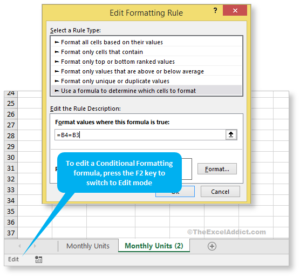
*** Note that, as I mentioned in a previous tip, editing a formula in the Conditional Formatting dialog can be tricky AND REALLY FRUSTRATING. You’ll have to click in the formula box then press the F2 key to switch from Enter mode to Edit mode, which will allow you to use the arrow keys to move the cursor around the formula box.
