Relative cell references

The dollar sign ($) in a formula – Fixing cell references

When you copy and paste an Excel formula from one cell to another, the cell references change, relative to the new position:

EXAMPLE:

If we have the very simple formula “=A1” in cell B1 it will change as follows when copied and pasted:

Pasted to B2, it becomes “=A2”

Pasted to C2, it becomes “=B2”

Pasted to A2, it returns an error!

In each case it is changing the reference to refer to the cell one to the left on the same row as the cell that the formula is in, i.e. the same relative position that A1 was to the original formula.

The reason an error is returned when it is pasted into column A, is because there are no columns to the left of column A.

This behavior is very useful and is what allows a sum to be copied across or down the page and automatically refer to the new column or row that it finds itself in.

But in some situations, you want some or all of the references to remain fixed when they are copied elsewhere.

The dollar sign ($)
This is where the dollar sign is used.

EXAMPLE:

Take an example where you have a column of Sales values in Pounds Sterling in column A and a formula to convert these into US Dollars in column B. You could enter the actual exchange rate into the formula but it would be more sensible to refer to a cell where the exchange rate is held, so that it can be updated whenever it is needed.

 

 

 

 

 

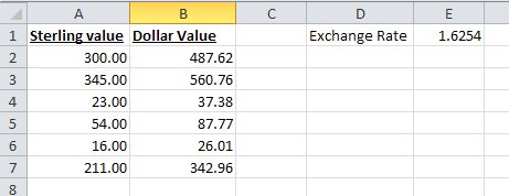
The simple formula for cell B2, would be “=A2*E1”, however, if you copy this down, then the formula in cell B3, would read “=A3*E2” as both references would move down a row as described above.

This is where the dollar sign ($) is used. The dollar sign allows you to fix either the row, the column or both on any cell reference, by preceding the column or row with the dollar sign. In our example, if we replace the formula in cell B2 with “=A2*$E$1”, then both the “E” and the “1” will remain fixed when the formula is copied. i.e. in cell B3, the formula will read “=A3*$E$1”, still referring to the cell with the exchange rate in it.

In this example, we have fixed both the row and the column, but in other situations, you may just want to fix one or the other, for example:

 

 

 

 

 

 

 

 

 

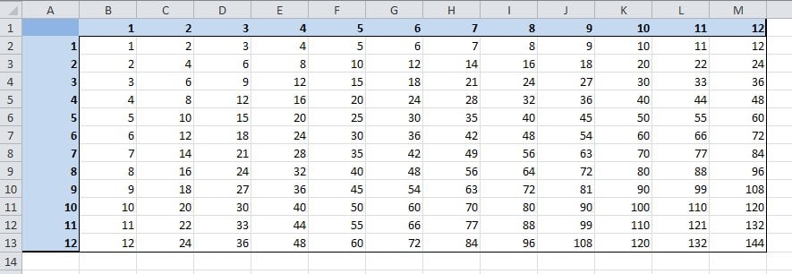
Above we have a spreadsheet calculating the times tables where we want to every cell in the white area to be the product of its row and column heading. This is easy using the dollar symbol. In cell B2, the formula without dollars would be “=A2*B1”, but for this formula to work when copied to each column, we need it to always look at column A for the first reference and to work for each row, we need to always look at row 1 for the second. Using the dollar sign to do this, it becomes “=$A2*B$1”. This can then be copied to every cell in the white area.